AI & Data Mining
Data Mining
Notes from the Data Mining course of the Master in Cyber Security at the University of Pisa: data representation, preprocessing, classification, clustering and association rules.
- Date
- Difficulty
- n/a
- Platform
- Master UniPi
- Reading
- 30 min
Course: Data Mining, Master in Cyber Security, University of Pisa (Prof. Francesco Marcelloni) Reference textbook: J. Han, M. Kamber, J. Pei, Data Mining: Concepts and Techniques, Morgan Kaufmann
Introduction
Data mining is the practice of searching large amounts of data for useful patterns and trends, that is, extracting models from data.
Machine Learning
-
Supervised learning: the model learns from labelled data; the labels supervise the learning process that builds the model.
- Classification models: the desired output is one of a few possible classes (e.g. an email is spam or not spam; hair is blond, brown or red).
- Regression models: the output is a number, so there are many possible outputs.
-
Unsupervised learning: the data is not labelled; the goal is to find out whether the available data can be grouped in some way, discovering patterns and structures in it.
- Clustering models: algorithms that analyse unlabelled data and find patterns based on the characteristics of the data (e.g. user profiling).
-
Reinforcement learning: does not need data up front; learning comes from the interaction between an agent (software) and its environment (often used in robotics through sensors). The model learns by taking actions and interpreting the feedback each action produces.
-
Semi-supervised learning: uses unsupervised learning to cluster the data and then supervised learning to label the clusters found.
Malware Detection
Data mining can be used to detect malware on a system.
- Anomaly detection: data mining builds a model of the normal behaviour of the monitored system. When the real system differs significantly from this “virtual” model, we can suspect anomalous behaviour and therefore possible malware.
- Misuse detection: identifies known attacks with a model built from examples of past attacks, using classification models (supervised learning).
- Hybrid approach: combines classification and anomaly detection to improve the detection of attacks.
Intrusion Detection
Malicious actors trying to carry out attacks can be detected by analysing system logs and identifying anomalies that correspond to the attack.
Fraud Detection
For example, by learning how a credit card is normally used, we can detect behaviour that deviates from its usual use.
Today AI/ML techniques turn text into numeric vectors:
- Example: “mouse”
- It means both the animal and the computer device.
- Looking at the string alone, the meaning is ambiguous.
- If we represent “mouse” in the context where it is used, current AI/ML techniques map it to a different numeric vector depending on that context.
- Once we have a numeric description that depends on the context, we can apply data mining algorithms.
Data Representation
A data set is a collection of data objects.
Object: a generic entity, such as a user, a product sold, a patient, etc.
- Each object is described by a number of attributes.
- In database terms, each object is a row of a table and each attribute is a column.
Attribute: a field that describes a characteristic of the object.
- E.g. name, address, date of birth, student ID.
Main attribute types
Nominal:
- An attribute that represents a category, a state or a “label”.
- These attributes take few values (e.g. hair colour, zip code, occupation).
- Unlike numeric values, labels cannot be ordered.
- Measuring distance is not trivial. Suppose two “person” objects are described by the attributes “eye colour” and “hair colour”, and we want to find the most similar people based on these two attributes. The distance for nominal attributes is defined as follows:
-
Given two objects and , the distance is
-
: number of nominal attributes describing each object
-
: number of attributes on which the two objects have the same value
Example: p1 = (green, blond), p2 = (green, black)
-
Binary:
- A nominal attribute that only takes the values or .
- Binary attributes can be symmetric or asymmetric:
- Symmetric: both values are equally likely and equally important.
- Asymmetric: one value (usually 0) is much more frequent than the other, and the rare value is the one that matters.
- The distance between two objects with binary attributes is computed from a contingency table:
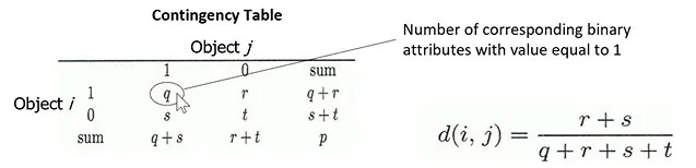
: number of attributes equal to in both and
: number of attributes equal to in and in
: number of attributes equal to in and in
: number of attributes equal to in both and
: total number of attributes
Distance for symmetric binary attributes:
- Note that .
- With asymmetric attributes, in practice:
-
is very large;
-
as a result the two objects look very close (distance close to 0);
-
so for asymmetric attributes we ignore , and the distance becomes:
-
Ordinal:
-
A nominal (“label”) attribute whose values have a meaningful order.
-
For example, for sizes we perceive an order:
-
We want the distance to reflect this order (small, medium, large):
-
map the possible values to increasing integers, in this case 1 = small, 2 = medium, 3 = large;
-
then normalize the range of each attribute to , mapping 1, 2, 3 so that the ordinal attribute takes values between 0 and 1;
-
with the formula:
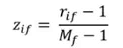
Where:
- is the rank of the value of attribute for object , after mapping the labels to increasing integers
- is the number of ordered states that attribute can take
-
In this example:
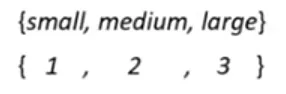
-
where 1 = small, 2 = medium, 3 = large
-
-
which gives:
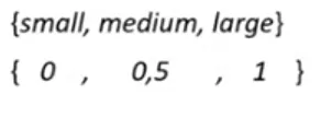
-
-
-
This turns a nominal attribute (small, medium, large) into a numeric one (0, 0.5, 1), so numeric distances can be used.
Numeric:
Numeric attributes can be:
- Interval-scaled:
- measured on a scale of equal-sized units;
- they have no true zero point;
- e.g. temperature in degrees Celsius: 0 °C is a conventional zero, not the absence of temperature;
- this means that addition and subtraction are meaningful, but multiplication and division are not.
- Ratio-scaled:
- e.g. temperature in kelvin, lengths, amounts of money;
- they have a true zero, so multiplication and division are meaningful (10 K is twice as hot as 5 K).
To compute the distance between objects described by numeric attributes:
- we can use the Minkowski distance, which is the Euclidean distance when h = 2 and the Manhattan distance when h = 1.

- Objects are essentially points in an -dimensional space, one dimension per attribute, so the Euclidean distance (h = 2) tells us how far apart they are.
When an object is described by attributes of different types, the distance is computed for each attribute (normalized to ) and then combined as a weighted average:
where if attribute is missing for or (or if it is an asymmetric binary attribute equal to 0 for both), and otherwise.
Measuring data dispersion
It is generally useful to understand how attribute values are distributed in the data set.
Box plot:
-
It is based on percentiles: the -th percentile of a set of numeric values is the value such that % of the values are less than or equal to (e.g. the median is the 50th percentile).
-
The box plot uses quartiles:
- Q1 = 25th percentile
- Q2 = 50th percentile (median)
- Q3 = 75th percentile
-
It shows the distribution of the values of a numeric attribute.
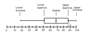
- Lower extreme = minimum
- Lower quartile = Q1
- Median = Q2
- Upper quartile = Q3
- Upper extreme = maximum
- Whiskers: the two lines outside the box
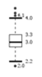
Outliers (the asterisks in the chart) are points that are very different from the rest of the data set, typically more than 1.5 × IQR (Q3 − Q1) beyond the quartiles.
A box plot shows where the values are concentrated and, above all, how spread out they are within the attribute.
Histogram:
Another option is the histogram, which shows how often the values fall into each range.
- In a histogram the area of each bar represents the frequency of the range, while in a bar chart the height carries the information. When all ranges have the same width, area and height give the same information, so a histogram is usually read like a bar chart.
- A histogram gives much finer detail than a box plot, which only summarizes the data with quartiles.
- Box plots and histograms show how the values of a single attribute are distributed.
- To understand whether, given two attributes, one grows when the other grows (or decreases), we use a scatter plot.
Scatter plot:
-
Each object is drawn as a point on a Cartesian plane, using the values of two of its attributes.
-
One attribute goes on the x axis and the other on the y axis.
-
Scatter plots make it easy to see whether two attributes are related. If two attributes describing an object are strongly correlated, they carry the same information and one of them may be redundant for the problem we want to solve. So if a correlation analysis shows that two attributes are strongly correlated, we can decide to drop one of them.
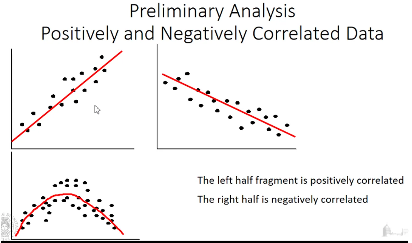
- In the first scatter plot, y grows as x grows: the points lie close to a line.
- The second shows the opposite trend.
- Both show a correlation between the two attributes: as one grows, the other grows (or decreases), so the two attributes carry similar information.
- Attributes with the same trend probably have the same informative value, so a data mining technique could use only one of them.
- The bottom scatter plot is different: the points do not follow a line, the correlation is positive up to a certain value of x and negative after it.
This correlation analysis helps find pairs of redundant attributes. Scatter plots can only be drawn for numeric attributes.
The Data Mining Process
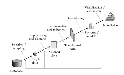
Whatever the problem, we follow the process shown above:
- We start from a set of data from which we want to extract new knowledge, such as patterns or models.
- Selection/sampling and preprocessing/cleaning: once the target data has been identified and collected, it may be inconsistent, redundant or dirty, so it has to be cleaned to make it homogeneous.
- Transformation and reduction: normalize the attributes (for example to the range 0–1) to make them easier to analyse, and remove the attributes that are redundant or not needed.
Data Cleaning
Data cleaning removes the noise from the data.
Common cases
- Incomplete data: some attributes of a data object are missing. This is a big problem because it pollutes the algorithms that compute the distance between objects.
- Noisy data: some values contain errors, unexpected values or outliers.
- Inconsistent data: attributes conflict with each other, for example two attributes expressing the same information with different values. Inconsistencies also appear when merging two databases that follow different conventions: one may store lengths in metres and another in inches without stating the unit.
- Intentionally noisy data: the data set forces some values, for example a default value that does not match the real one (also called disguised missing data).
Incomplete data: how to fix it
Three main approaches:
- Ignore the object with the missing attribute. This works if the share of objects with missing values is negligible. If it is high, removing them changes the distribution of the data and makes the model unreliable.
- Fill in the missing value manually. Rarely feasible, because today’s data sets are far too large.
- Fill in the missing value automatically, in one of several ways:
- Use a constant such as “unknown”, to explicitly flag that the value is missing.
- For numeric attributes, use the mean of that attribute.
- In classification, where each object has a class, use the mean of the attribute computed only on the objects of the same class: the estimate is more precise.
- Infer the most probable value from the other attributes of the object, again with a data mining technique (e.g. regression or a decision tree).
Noisy data: how to fix it
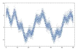
When applying a filter to reduce noise, keep the goal in mind. Filtering is fine to clean the data, but if we want to detect outliers the filter would remove them.
Rectangular smoothing filter: it “smooths” the signal. We choose a window, that is, a number of samples, and the filter replaces the central sample with the mean of the samples in the window.
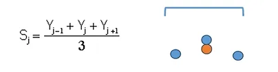
Smoothing filter over a window of 3 samples.
The result:
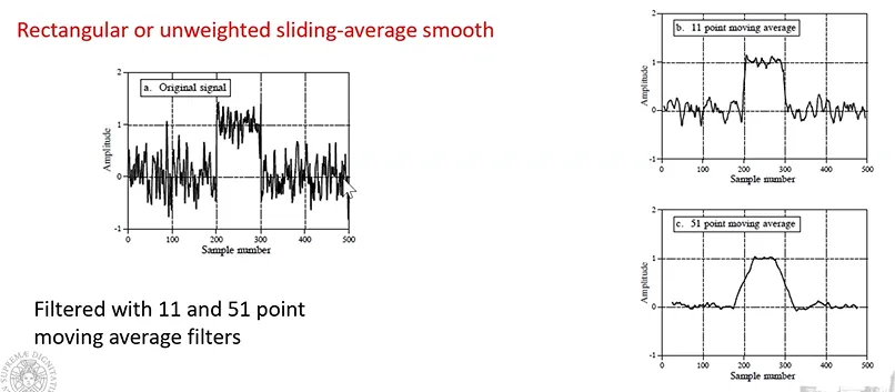
The image shows how much the window size matters: with a 51-sample window the signal changes significantly from the original one, while with an 11-sample window it does not.
The wider the window, the stronger the smoothing, but also the higher the risk of altering the signal (or the data set) itself. Which width works best depends on the goal.
Savitzky-Golay filter (generalization of the rectangular filter)
It computes a weighted average of the samples inside the window.
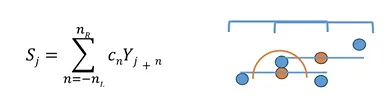
= number of samples to the left of the data point
= number of samples to the right of the data point
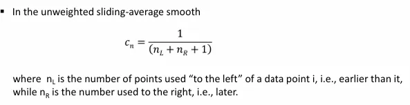
:
- if is constant, we get the usual rectangular filter, which approximates the samples in the window with a line parallel to the x axis;
- if we fit polynomials of higher order, we can model more closely how the samples move inside the window.
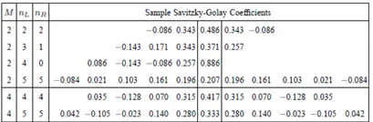
Savitzky and Golay computed the optimal coefficients for each polynomial order and window size.
The useful part is that these coefficients can be computed once, offline, for the chosen polynomial and then applied directly when filtering.
With a Savitzky-Golay filter the height of the peaks is preserved much better as the window grows, thanks to the polynomial fit.
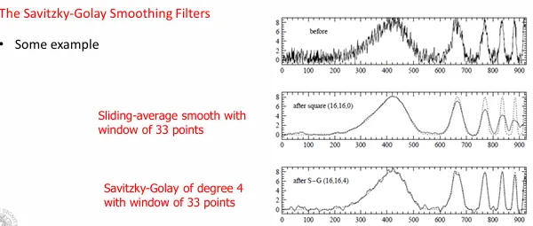
What is the best choice?
We use the smoothing ratio, the ratio between the window width and the width of the peak:
- if the goal is to measure the height and width of the peak, use smoothing ratios below 0.2;
- if the goal is to measure the position of the peak, higher smoothing ratios can be used.
When should we not use a smoothing filter?
- When we want to detect outliers.
Data discrepancy detection:
How can we tell whether the value of an attribute is plausible and not dirty?
- Use metadata (domain, range, distribution of each attribute).
- Check some rules:
- unique rule: each value of the attribute must be different from all the other values of that attribute;
- consecutive rule: there can be no missing values between the lowest and the highest value, and all values must be unique (e.g. invoice numbers);
- null rule: specifies how blanks, question marks or special characters that indicate a null value must be handled.
- Use tools:
- data scrubbing: uses simple domain knowledge (e.g. postal codes, spell checking) to detect and correct errors;
- data auditing: analyses the data to discover rules and relationships and detect values that violate them, for example finding redundant objects or attributes.
Redundancy:
- Replicated attributes: the same attribute or object appears more than once.
- Derived attributes: an attribute can be derived from another one (e.g. age from date of birth), so one of the two can probably be removed.
Correlation Analysis
The goal is to find redundant attributes, so that they can be removed without changing the output of the model.
Chi-square () is a statistical test to analyse the correlation between two nominal attributes.
It is based on the contingency table:
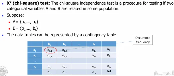
- rows: possible values of attribute A
- columns: possible values of attribute B
- each cell: number of instances in which A and B take the values of that row and column
compares the observed counts with the expected counts, where the expected counts are computed assuming the two attributes are independent:
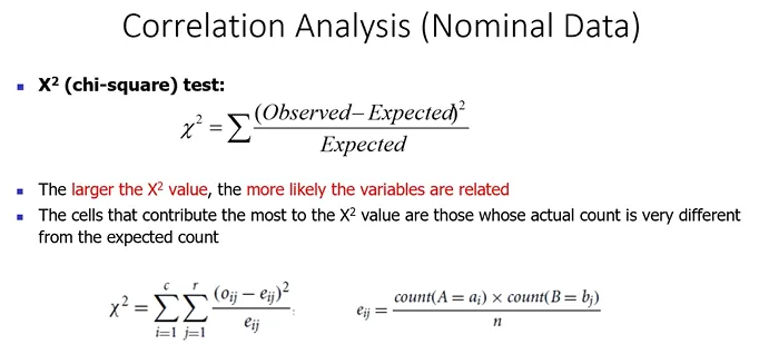
- If is small (close to 0), observed and expected counts are similar: the attributes are independent and we keep both.
- If is large, the attributes are correlated, so one of them is probably redundant and can be removed.
Example:
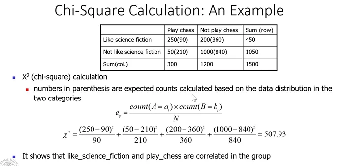
How do we decide whether the value of really means the attributes are correlated?
We choose a significance level and compute the degrees of freedom, , where and are the number of distinct values of the two attributes:
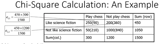
In this example there is 1 degree of freedom: we pick the significance level and read the critical value from the table.
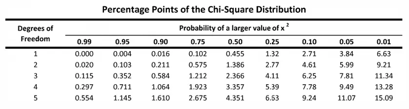
If the computed value is greater than the value in the table, we reject the independence hypothesis: the two attributes are correlated with the chosen confidence.
Pearson correlation coefficient (numeric attributes)
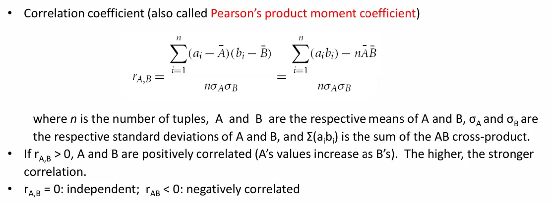
The sum of the products of the deviations from the mean is divided by the number of objects times the standard deviations of A and B. The coefficient ranges from −1 to +1:
- if it is greater than 0, the attributes are positively correlated;
- if it is 0, there is no linear correlation;
- if it is less than 0, the attributes are negatively correlated.
A coefficient close to ±1 means the two attributes carry similar information, so we can decide to remove one of them.
Data Reduction
- Dimensionality reduction: improves efficiency but above all the quality of the results. With many dimensions all points look far apart from each other, so they cannot be clustered (the curse of dimensionality). Reducing the number of dimensions helps.
- Numerosity reduction: only improves efficiency, reducing computation time.
- Data compression.
How can we reduce dimensionality?
Principal Component Analysis (PCA)
PCA looks for a transformation of the original space into a new space (new axes) such that, when the data is projected onto the new axes, the values are as spread out as possible. If the projections overlap, that axis does not represent a relevant dimension.
Mathematically, PCA computes the eigenvectors and eigenvalues of the covariance matrix of the data: the eigenvectors are the new axes (principal components) and the eigenvalues measure the variance of the data along each of them. PCA keeps the components with the highest variance and discards those with low variance, leaving only the dimensions that are useful to analyse the data set.
Heuristic search in attribute selection
Another way to reduce the number of features works directly in the original space.
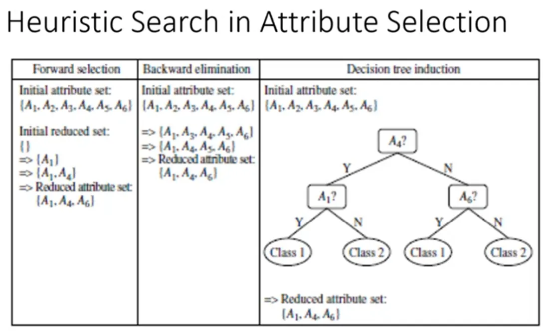
- Forward selection: start with an empty set of selected features and, at each iteration, add the attribute that is best at that point. To decide which attribute is best we need a metric to compare attributes.
- Backward elimination: start with all the attributes and, at each iteration, remove the worst one. Again, a metric is needed to decide which is the worst.
- Decision tree induction: not a feature selector but a classifier, which implicitly selects features (the attributes that do not appear in the tree are irrelevant).
Numerosity reduction: sampling
We keep a sample of the objects, which must be a reasonably faithful representation of the original data set.
- Simple random sampling without replacement: once an object is selected it is removed from the data set and cannot be drawn again.
- Simple random sampling with replacement: the selected object is not removed, so it can be drawn again.
- Stratified sampling: the reduced population keeps exactly the same class proportions as the original one.
Data Transformation
Normalization:
Min-max normalization: maps the attribute to a fixed range, for example between 0 and 1.

This normalization has a problem with outliers: if the minimum or the maximum is an outlier, all the other values are squeezed into a small part of the range, so the scale no longer reflects the data.
Z-score normalization (less sensitive to outliers):
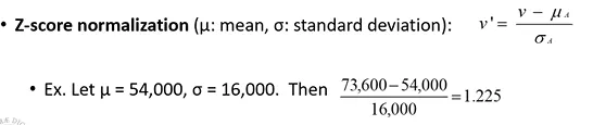
With z-score normalization the attributes do not all fall in the same fixed range, unlike min-max normalization; instead each attribute ends up with mean 0 and standard deviation 1.
Classification
Goal: assign a class to each object.
We start from a set of already classified data (the training set); when a new object arrives we must classify it.
A naive classifier: if the new object exactly matches an object in the training set, assign it the class of that object; if it matches none, we cannot classify it.
Lazy learners
1-nearest neighbour: assigns the class of the most similar (closest) object in the training set.
k-nearest neighbours: assigns the majority class among the closest objects; is essentially chosen by trial and error. It is computationally expensive, because the distance from the new object to every point in the data set must be computed.
- To reduce the computational cost we can reduce the number of objects in the training set:
-
Sampling: build the training set by sampling the original one.
-
Replacement: replace a group of objects with a single representative object.
-
Editing: reduce the number of objects while also improving the training set, by removing the objects that are useless or harmful:
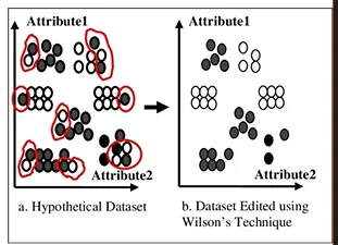
- Wilson’s editing uses the classifier itself:
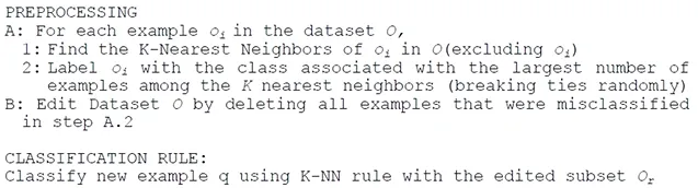
- apply k-nearest neighbours to each object of the training set: if the predicted class matches the object’s class, keep the object;
- if k-nearest neighbours returns a different class, remove the object, because it is probably noise in the training set.
-
These approaches need a lot of memory, since they have to keep and scan the whole training set.
Eager learners
We build a classification model and then use only the model, without going back to the training set as lazy learners do.
- The model is usually simple to evaluate, so classification is very fast.
- We must, however, estimate how accurately the model classifies objects:
- we build a test set, separate from the training set, in which the correct class of each object is known, and use it to evaluate the classifier;
- accuracy is the percentage of test samples that are classified correctly;
- overfitting: when the accuracy on the training set is much higher than the accuracy on the test set, the classifier has learned the training data too closely and will not work well on new objects.
Ways to build a classification model:
-
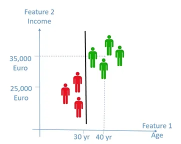
Separating line / Support Vector Machine (SVM):
-
The model is the equation of a line (a hyperplane in more dimensions): objects are classified according to the side of the line they fall on.
-
There is a problem, though:
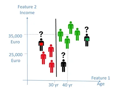
with this line, the new object is misclassified.
-
So the line must be chosen as the optimal one, which separates the classes with the maximum margin, equidistant from the closest points of each class (the support vectors).
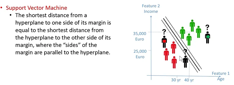
-
A linear classifier only works if the classes are linearly separable, which rarely happens in practice; SVMs handle this with soft margins and kernels, which map the data to a higher-dimensional space where it becomes separable.
-
SVMs are binary classifiers. For problems with more classes we train several of them, for example one per class against all the others (one-vs-rest).
-
-
Decision tree:
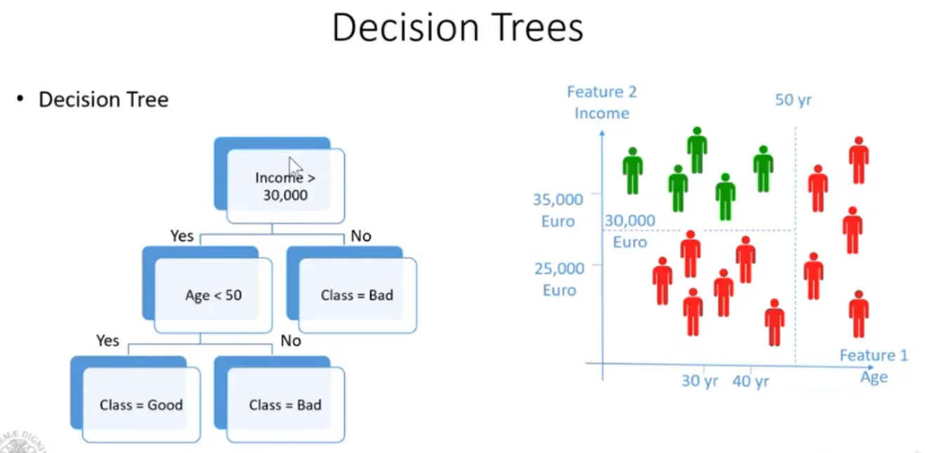
- An explainable classifier: we can see how it reaches its decision.
- It starts from a root node; each internal node is a test on the value of an attribute.
- The leaves are the classes.
- To classify an object, we walk the tree from the root down to a leaf.
- Classifying an object is like explaining how the classifier makes its decision.
- But how do we build the model?
Decision tree learning
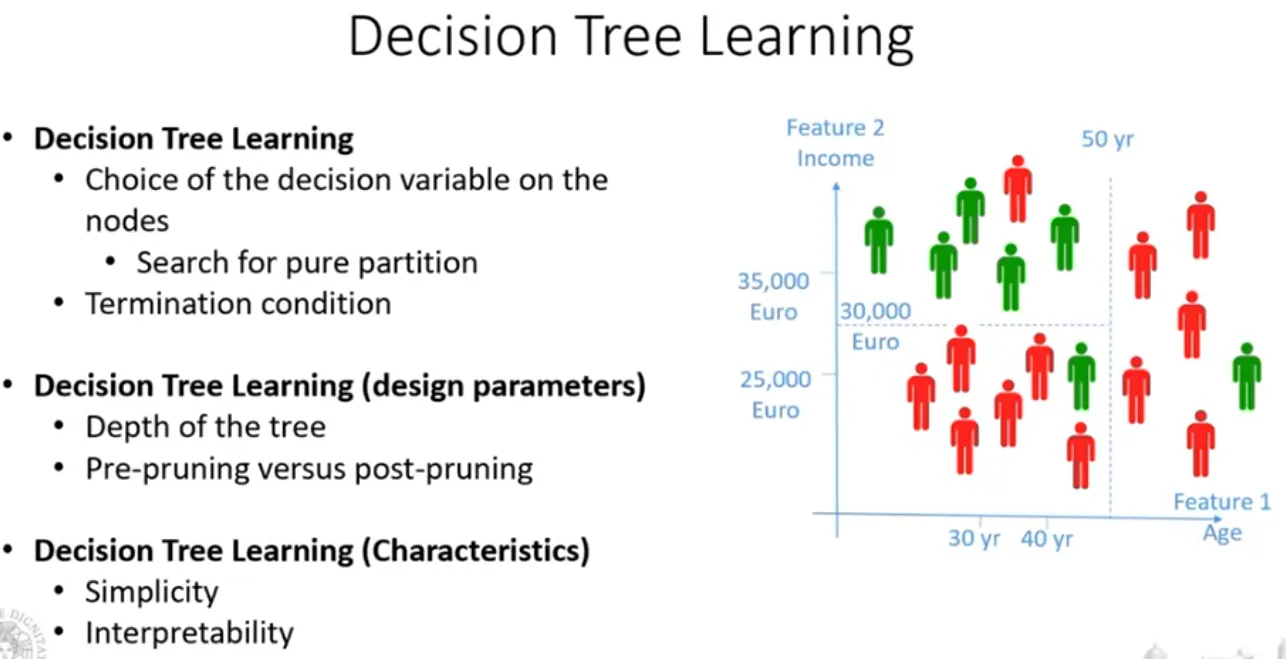
The algorithm must decide which attributes to use in the decision nodes and in which order: which attribute goes in the root and which in the following branches.
The idea is to choose attributes that split the data into sub-spaces containing a single class.
In the real world we cannot always find a sub-space with a single class. When the attributes run out, we create a leaf labelled with the majority class of the points that fall into that sub-space.
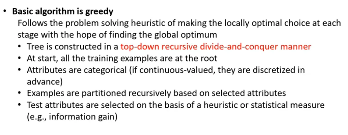
The algorithm builds the tree recursively, making the locally optimal decision at each level (greedy):
- Start with a root node containing all the training instances.
- Look for the attribute that best splits the node into child nodes.
- The attribute is chosen so that it splits the set into subsets that are as “pure” as possible, that is, with instances of the same class.
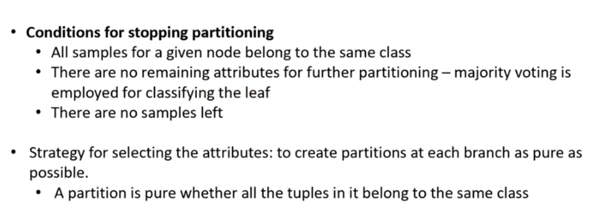
The algorithm stops when:
- all the instances in a node belong to the same class, so there is no point in splitting it further;
- there are no attributes left to split on: the node becomes a leaf labelled with the majority class;
- there are no instances left to split.
How do we choose the attribute?
- Information entropy:
-
suppose there are classes;
-
the probability of each class is estimated as the number of instances of that class divided by the total number of instances in the training set;
-
entropy is computed as follows:
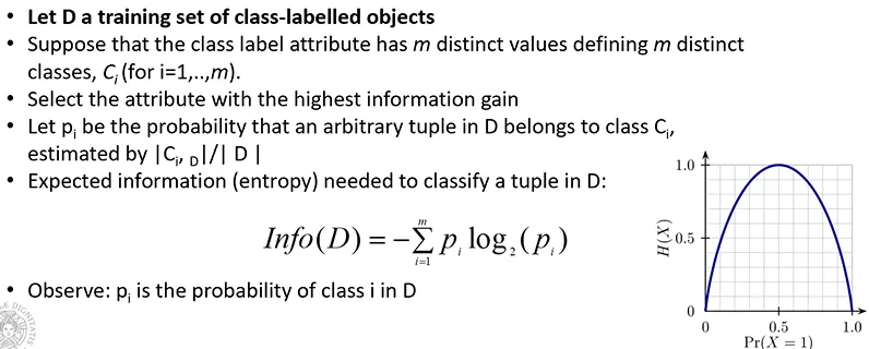
Y axis: entropy
X axis: probability of one of the two classes
-
entropy = 0 means the (sub)set contains a single class;
-
with two classes, entropy reaches its maximum of 1 when both classes are equally likely, with no prevalence of one over the other (with classes the maximum is ).
-
So when building the decision tree we select the attribute whose split produces the lowest entropy, that is, the highest information gain.
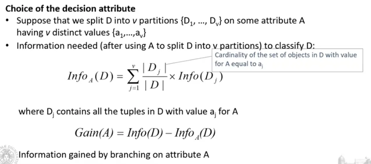
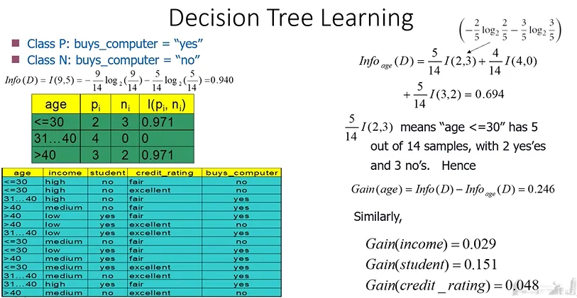
We compute the entropy of the initial data set, then for each attribute we look at how it splits the data into subsets and compute the weighted entropy of those subsets. The gain is the difference, and we select the attribute with the highest gain.
For example:
Performance Evaluation
To evaluate performance we need a test set in which the class of every instance is known.
The most intuitive metric is classification accuracy:
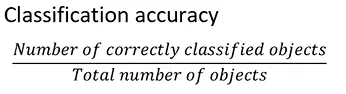
It looks suitable, but consider this example:
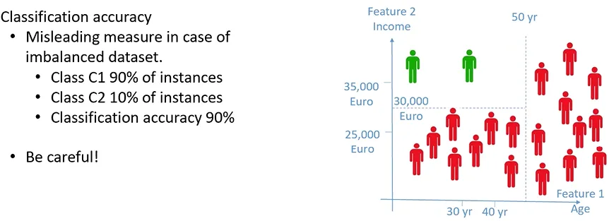
The data set is imbalanced: most instances belong to one class and only a few to the other.
Here the accuracy is 90%, but because of the imbalance even a classifier that assigns every instance to C1 would reach 90%. Accuracy does not really tell us how the classifier behaves, because it is dominated by the majority class.
Confusion matrix
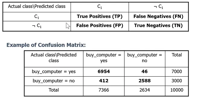
We build the confusion matrix shown above:
- TP: instances classified as C1 that belong to C1
- FP: instances classified as C1 that do not belong to C1
- FN: instances not classified as C1 that belong to C1
- TN: instances not classified as C1 that do not belong to C1
A perfect classifier produces a diagonal matrix, with FN and FP equal to 0.
Comparing confusion matrices
Comparing confusion matrices is not trivial, so we use different metrics depending on whether the data set is balanced:
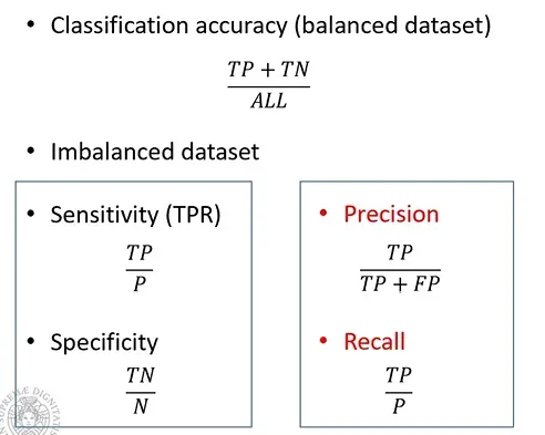
These metrics range between 0 and 1:
- Sensitivity (recall, true positive rate): 1 if every positive instance is classified correctly, 0 if none is.
- Specificity (true negative rate): 1 if every negative instance is classified correctly, 0 if none is.
Both sensitivity and specificity are needed to judge the quality of a classifier. The same applies to precision and recall.
F-measure
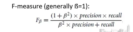
To compare two classifiers we can build their confusion matrices, compute precision and recall, and combine them into the F-measure (their harmonic mean):
Each classifier can also be drawn as a point in the ROC space:
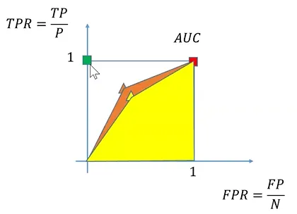
The two classifiers, the orange and yellow triangles, are placed in the ROC space after testing them on the test set and computing their confusion matrices, where:
- X axis: FPR, the ratio between FP and the number of negatives N
- Y axis: TPR, the ratio between TP and the number of positives P
The ideal classifier has:
- FPR = 0
- TPR = 1
so it is the green point at the top of the Y axis.
Our classifiers are the two triangles. For each one we draw the polygon that joins its point to (0,0) and (1,1): the classifier with the larger area under the curve (AUC) is the closer to the ideal one.
Performance evaluation on multi-class problems
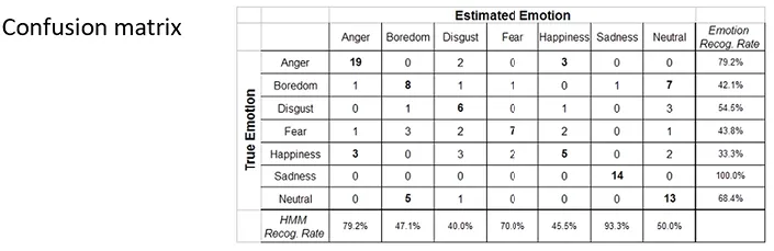
To compute TP, TN, FP and FN for a single class , we treat as the “positive” class and all the other classes as “negative”, reducing the problem to the two-class case seen above.
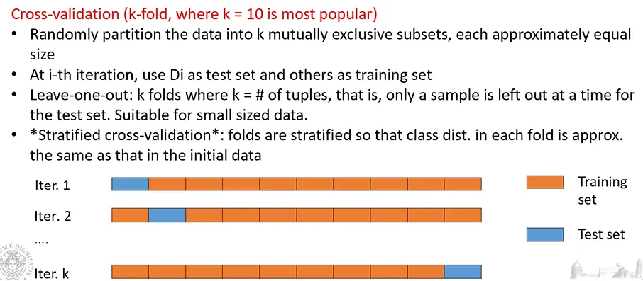
K-fold cross-validation
A single evaluation on a single test set may not be enough to judge the quality of a classifier.
Ideally we would have several data sets, using some for training and others for testing.
To do this with one data set we use k-fold cross-validation: the data is split into folds, and each fold is used once as the test set while the other are used for training.
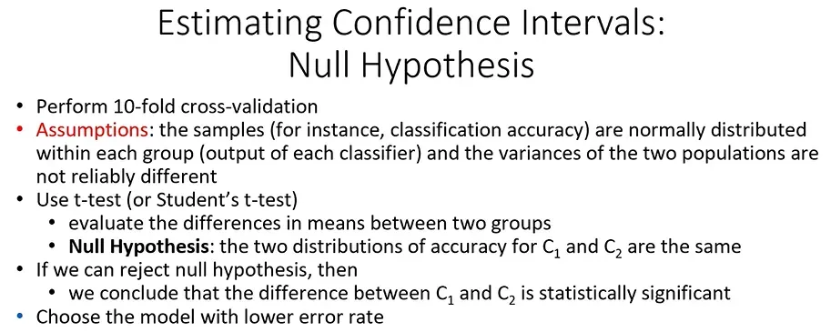
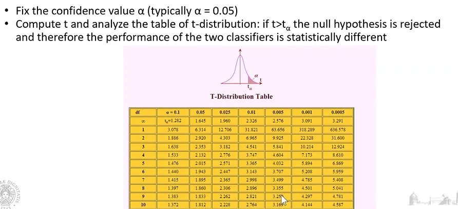
T-test
To compare two classifiers over the folds, if we can assume the differences are normally distributed and the variances across folds are similar, we can use the paired t-test:
Wilcoxon test
When we cannot make any assumption about the distribution, we use the Wilcoxon signed-rank test (non-parametric):
Classification in the Real World
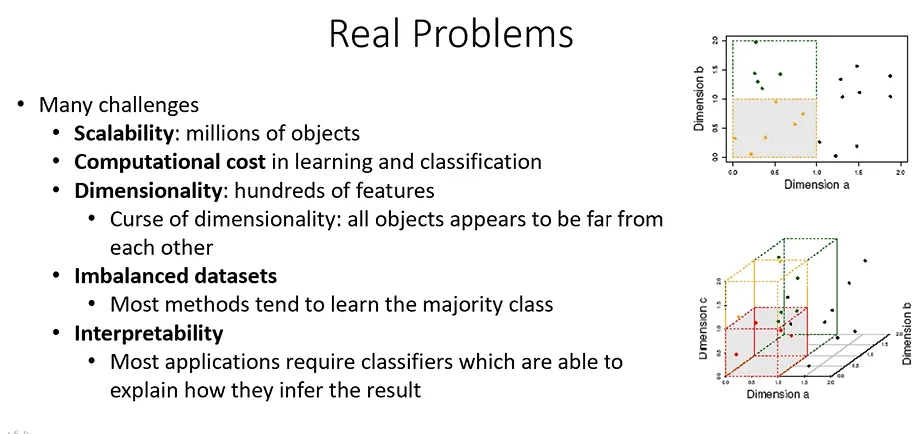
Today deep learning is the most common approach: models with many layers of interconnected neurons. They are powerful because their many parameters can be tuned to the problem at hand, but they need a lot of data.
Clustering
We have a set of objects, each described by attributes (features), but without any label.
The goal of clustering is to find out whether there is some structure in the data, so that the objects can be grouped according to some criterion.
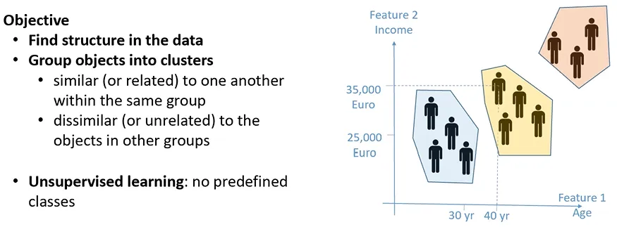
In general, objects that are similar to each other should end up in the same group:
- When can two objects be considered similar?
- When their distance is small.
So clusters should be compact and well separated from each other.
K-means
K-means uses the Euclidean distance as its similarity measure.
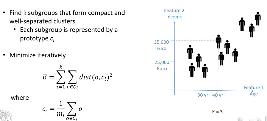
The algorithm minimizes the cost function , the sum of the (squared) distances between the objects of each cluster and the object that represents the cluster:
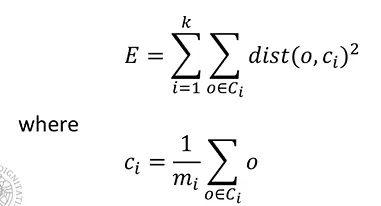
- : number of clusters we want to find
- : Euclidean distance
- : the objects that belong to cluster
- : the centroid of cluster
-
the mean of all the objects in the cluster, the object that represents it:
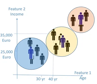
-
Pseudo-code
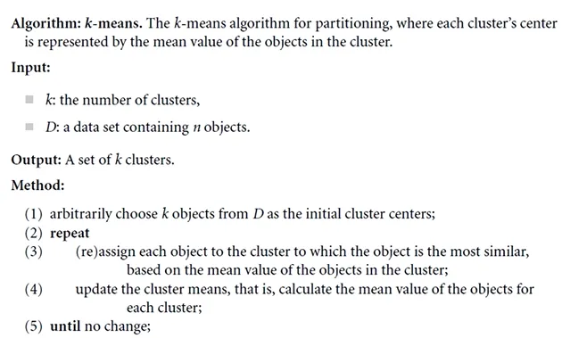
Issues
- The initial centroids are chosen at random. The cost function has local minima, so a bad initialization can lead to a poor result.
- A common fix is to run k-means several times and keep the solution with the lowest cost (or use smarter initializations such as k-means++).
- Other methods exist in the literature but are computationally expensive.
- An outlier can pull the centroid of its cluster towards it.
- To reduce this effect we can use the most central object of the cluster, the medoid, instead of the mean (k-medoids).
- Because it uses the Euclidean distance, k-means finds spherical (convex) clusters.
- We must choose , the number of clusters we expect, in advance.
Elbow method
Run k-means with a small , then increase step by step, recording the value of the cost function at each step.
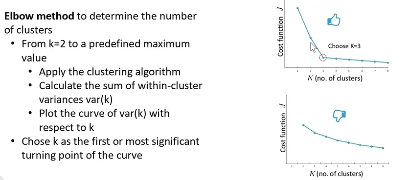
At the end, pick the at the “elbow” of the curve of the cost function.
If the data has no natural clusters there will be no clear elbow: k-means will still find “artificial” clusters, but they will not be very meaningful.
Density-based clustering
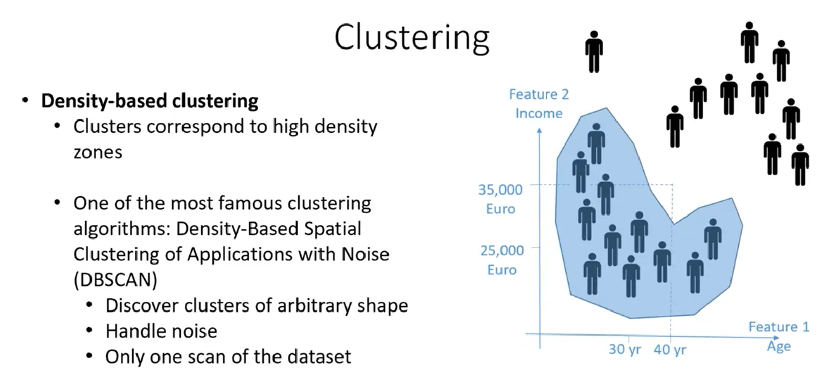
The idea is to find clusters as dense regions of the data, separated by regions with no points or with a low density of points.
DBSCAN
- It finds clusters of any shape, because it follows the density of the data.
- It handles noise well, because outliers end up isolated.
- It is not iterative: a single scan of the data set provides all the information needed to build the clusters.
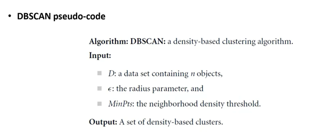
It needs two parameters, which express our notion of density:
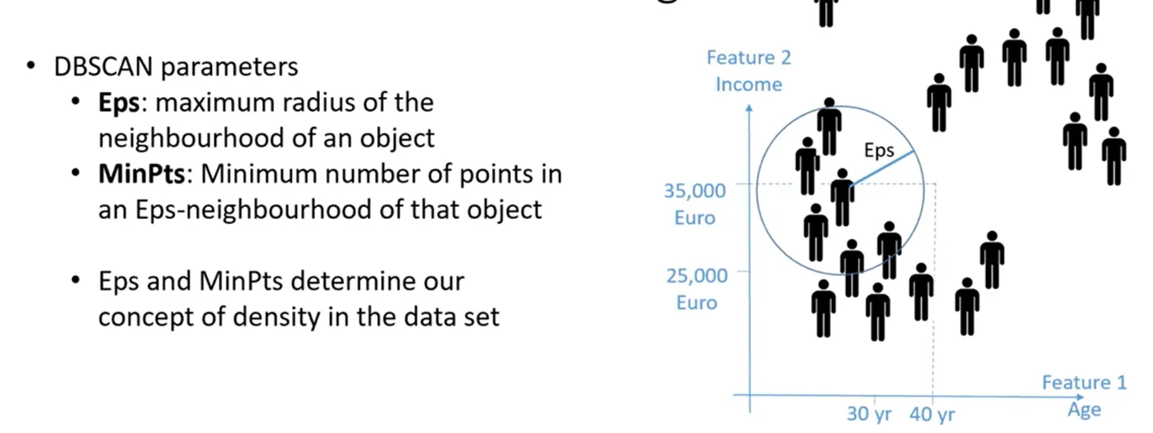
- Eps (epsilon): the radius of the neighbourhood of an object, that is, the maximum distance within which other objects are considered neighbours.
- MinPts: the minimum number of points in the neighbourhood of an object for that region to be considered dense, and therefore part of a cluster.
What these parameters identify:
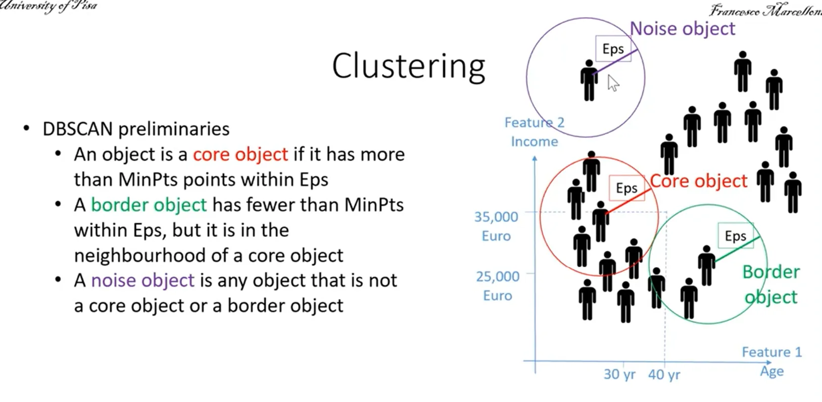
Core object: has at least MinPts points within its Eps-neighbourhood, so it lies in a dense region.
Border object: has fewer than MinPts points in its neighbourhood, but lies in the neighbourhood of a core object.
Noise object: neither core nor border; an isolated object, an outlier.
The DBSCAN algorithm
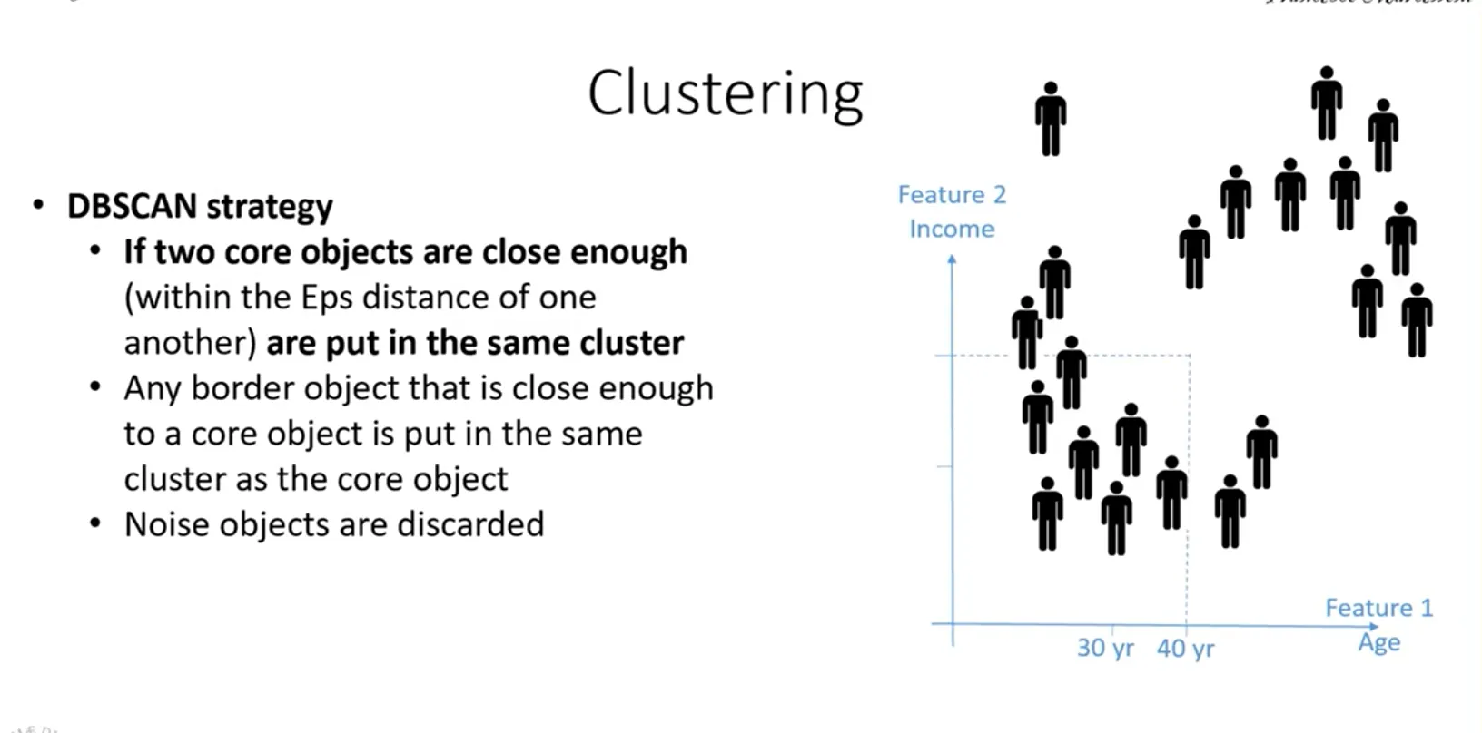
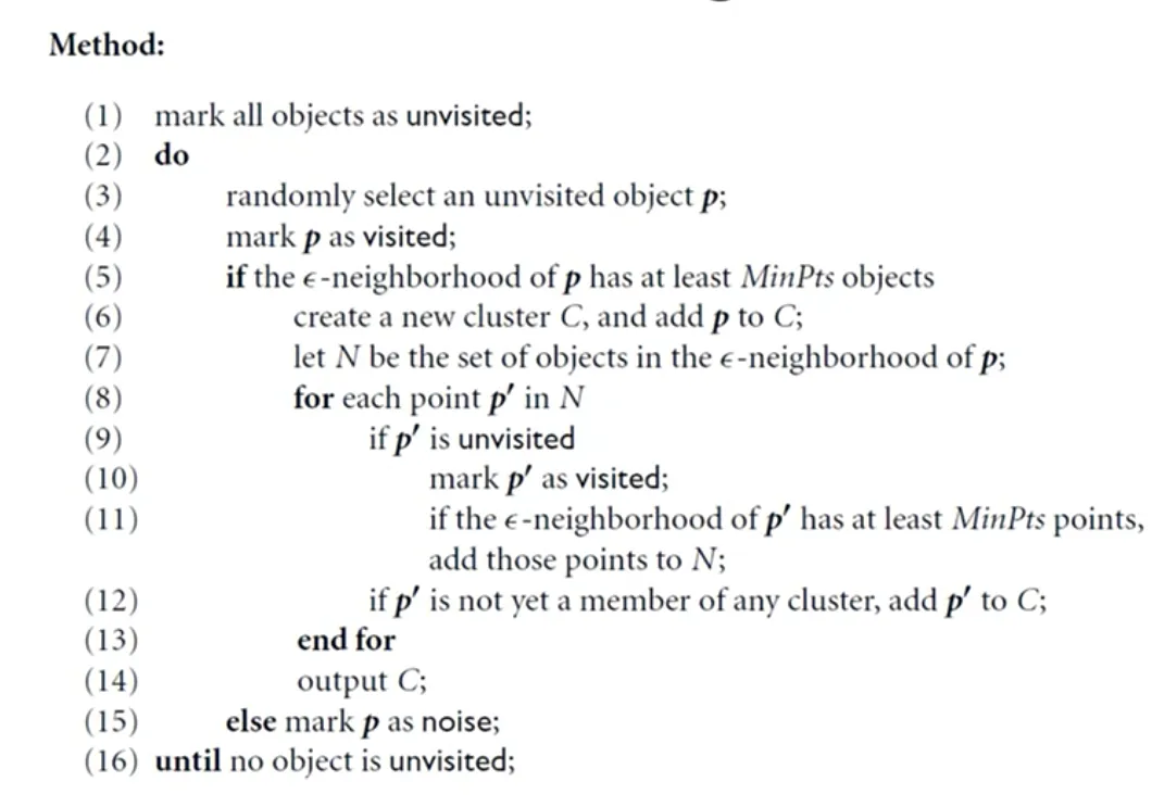
The algorithm picks an arbitrary object. If it is a core object, a new cluster starts: all the objects in its neighbourhood are added, and the neighbourhoods of the core objects among them are expanded in turn, until only border objects remain at the edges of the cluster. Then it moves on to the next unvisited object.
DBSCAN vs K-means
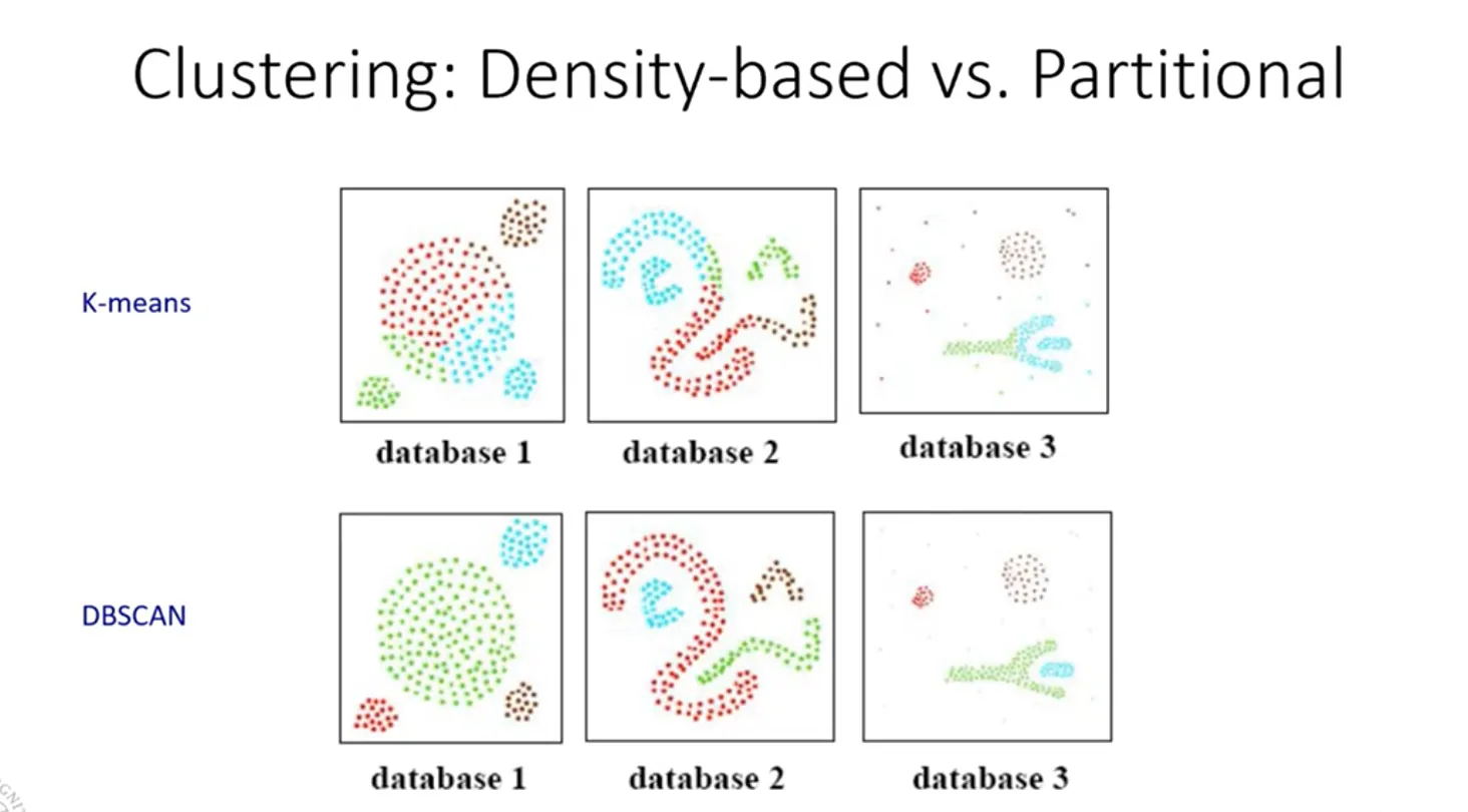
With DBSCAN, however, the parameters must be chosen carefully:
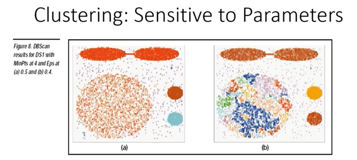
DBSCAN issues
- It is very sensitive to the choice of the parameters.
- If the whole data set has the same density, a good combination of parameters can be found. But if the clusters have different densities, no single pair of Eps and MinPts works for the whole space.
- So it works well when the natural clusters have similar densities.
How to choose Eps and MinPts
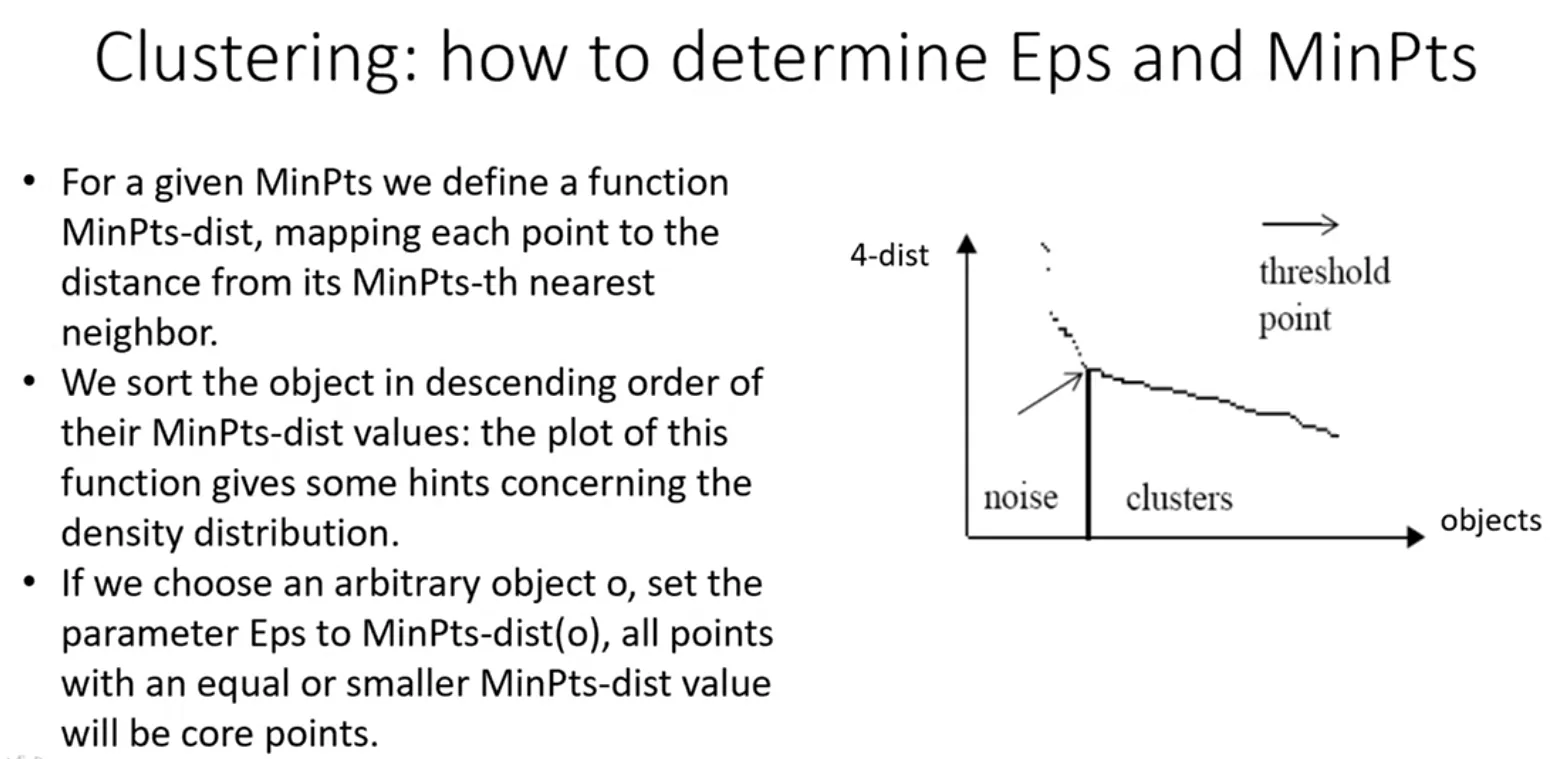
- Fix a value for MinPts and look for the best Eps for it.
- For each point, compute the distance to its MinPts-th nearest neighbour: with MinPts = 4, the distance to the 4th nearest neighbour.
- Do this for all the points and plot these distances, sorting the points in descending order of distance.
- The result should look like the plot above. If Eps is set at the elbow (the arrow), all the points to its right are core objects, because they have at least 4 points within the Eps radius. The points to the left are not necessarily outliers: they may also be border objects.
- Choose an Eps for which border and noise objects are only a small part of the data set.
Hierarchical Clustering
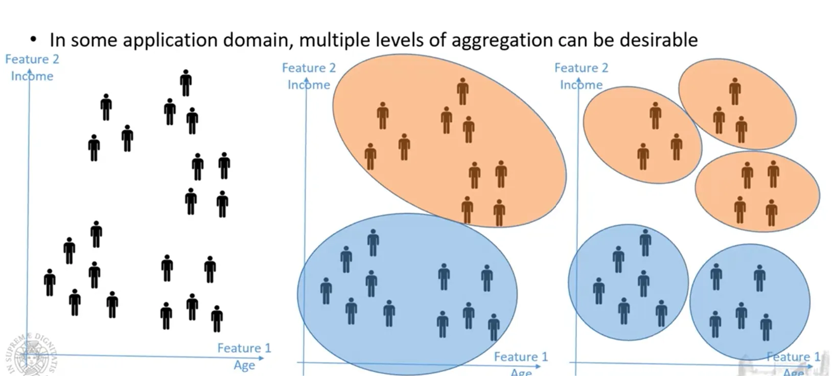
Hierarchical algorithms build a hierarchy of clusters.
They create partitions of the data at different levels of detail, from one large cluster down to more and more specific ones.
Agglomerative approach
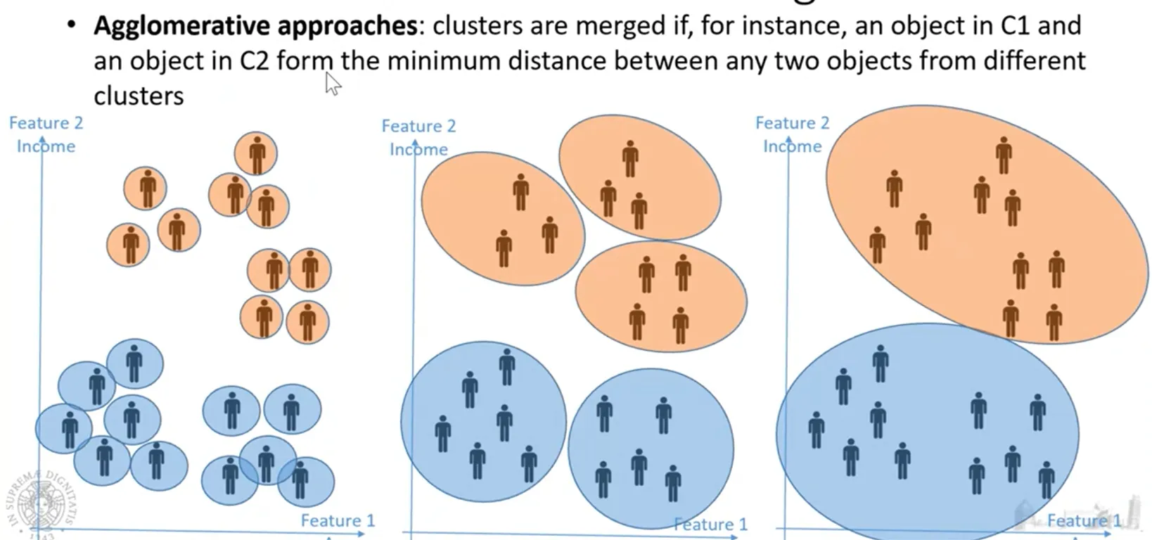
Start with one cluster per point and, at each step, merge the two closest clusters. This requires a distance between clusters (e.g. single, complete or average linkage).
Divisive approach
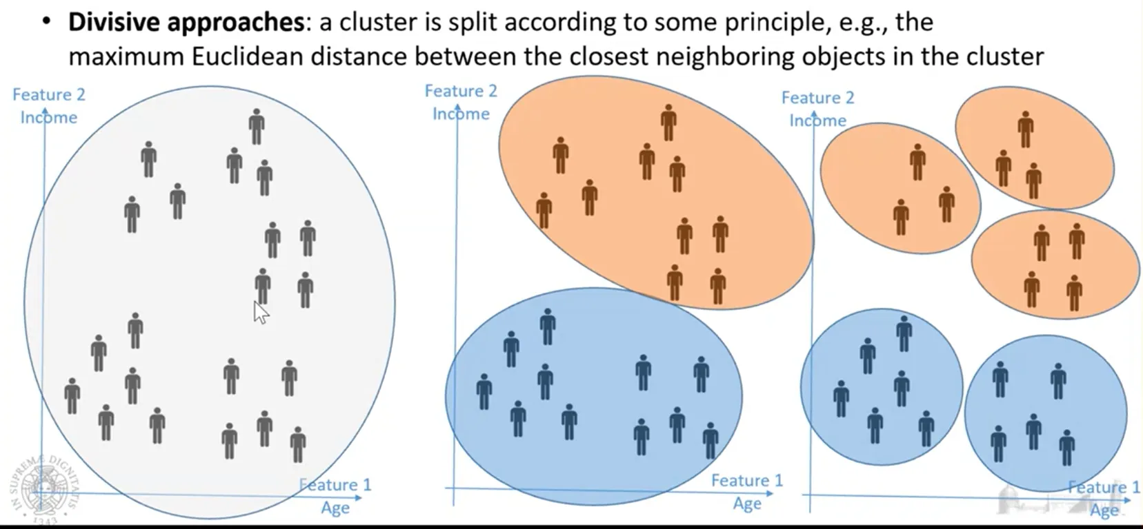
Start with the whole data set in a single cluster and split it into smaller and smaller sub-clusters.
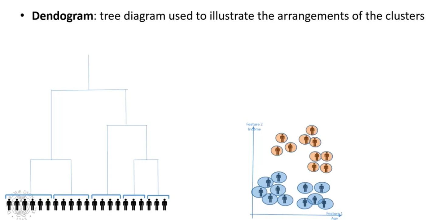
Dendrogram
A tree that shows how the clusters are organized hierarchically; cutting it at a given height gives a partition.
Clustering Metrics
How can we tell which clustering algorithm is working best?
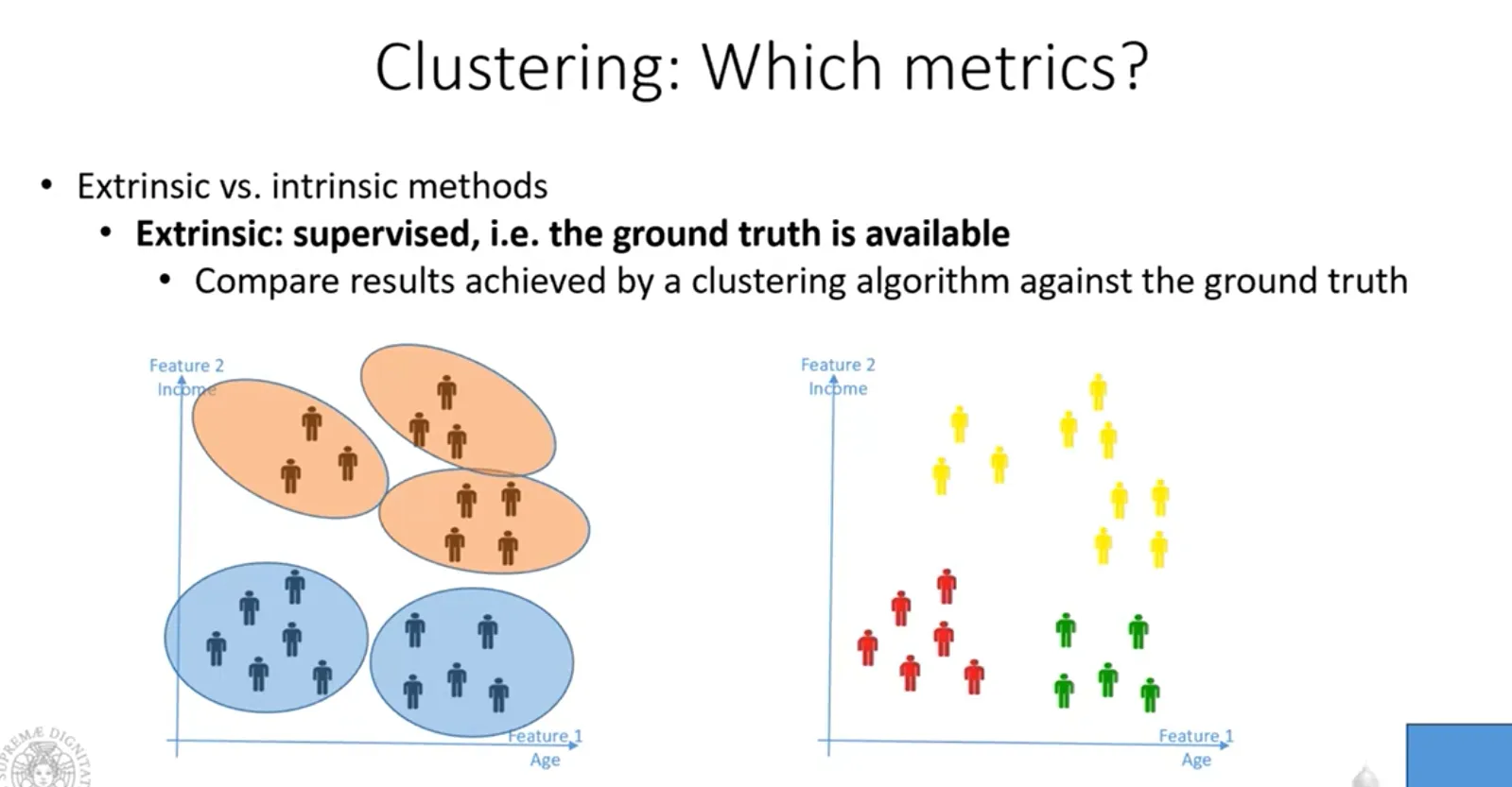
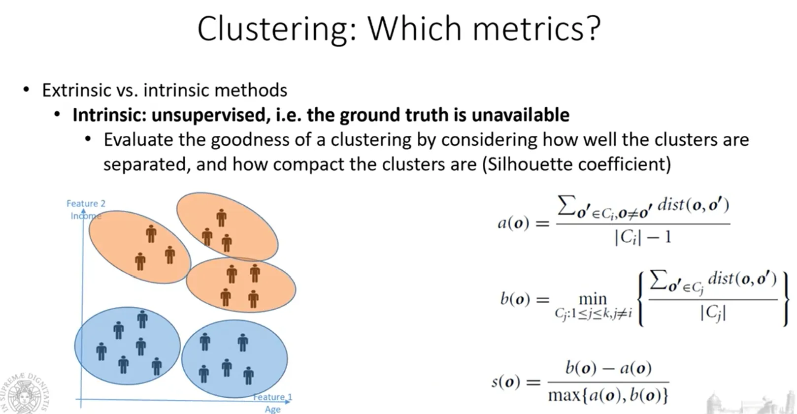
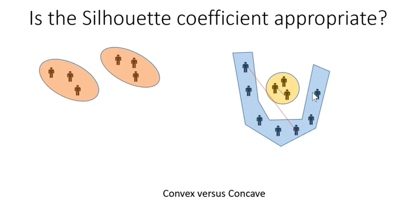
The silhouette coefficient only works well if we can assume the clusters are convex. With concave clusters it is no longer reliable.
Graph Clustering
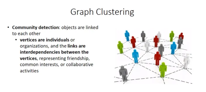
Graphs can represent the relationships in social networks: people are nodes and their relationships are edges, and we look for groups of nodes that are strongly connected to each other.
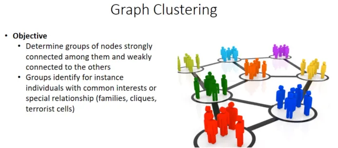
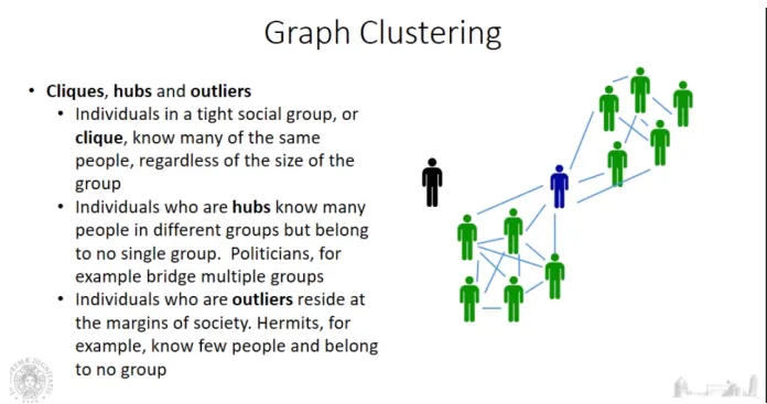
There are typically three kinds of nodes:
- clique (cluster) members: nodes that belong to a cluster;
- hubs: nodes connected to many clusters without belonging to any of them (in blue in the figure);
- outliers: nodes at the margins, with few connections.
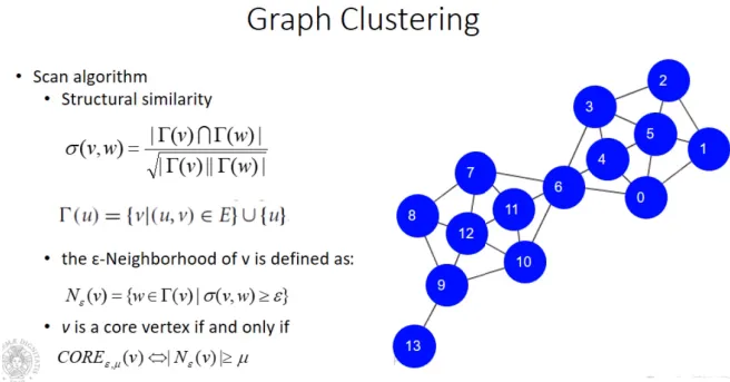
Two families of algorithms identify cliques, hubs and outliers:
- algorithms that define a similarity function between nodes and then apply traditional clustering algorithms;
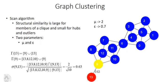
- algorithms that work directly on the graph, such as SCAN (Structural Clustering Algorithm for Networks). It is similar to DBSCAN, but density is not measured with Eps and MinPts on distances: it is measured by how strongly a node is connected to other nodes (structural similarity of their neighbourhoods).
Outliers
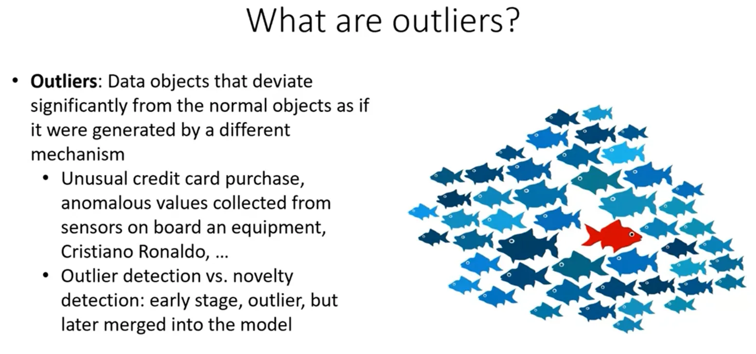
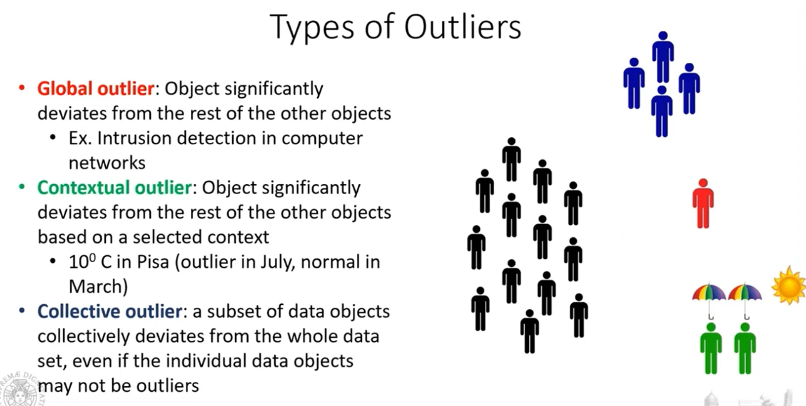
An outlier is an object that deviates significantly from most of the objects in the data set.
We must not confuse an outlier with a novelty, something new: a novelty starts as an outlier, but then more and more objects appear close to it.
Types of outliers
Detecting outliers
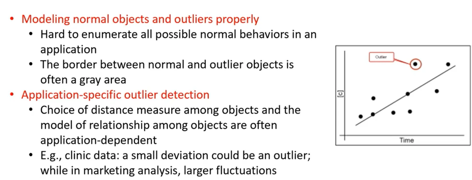
We model what normal objects look like and then measure how much each object deviates from that normal behaviour. In the example, the objects can be modelled with a least-squares linear fit: the line is the model of normal objects. If, computing the distance of every object from the line, some objects are very far from it, those are outliers.
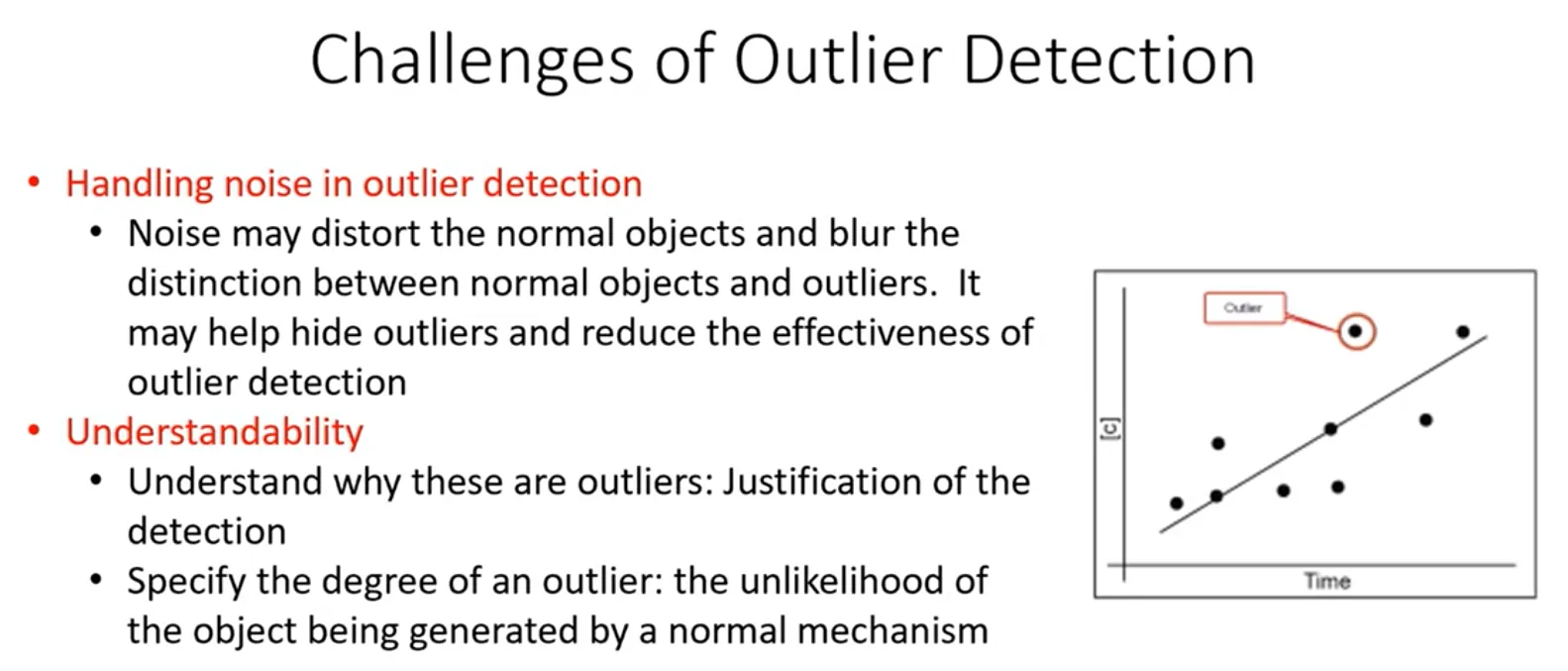
If we are interested in outlier detection, a smoothing filter changes the signal itself and may hide the outliers we are looking for.
Clustering-based detection
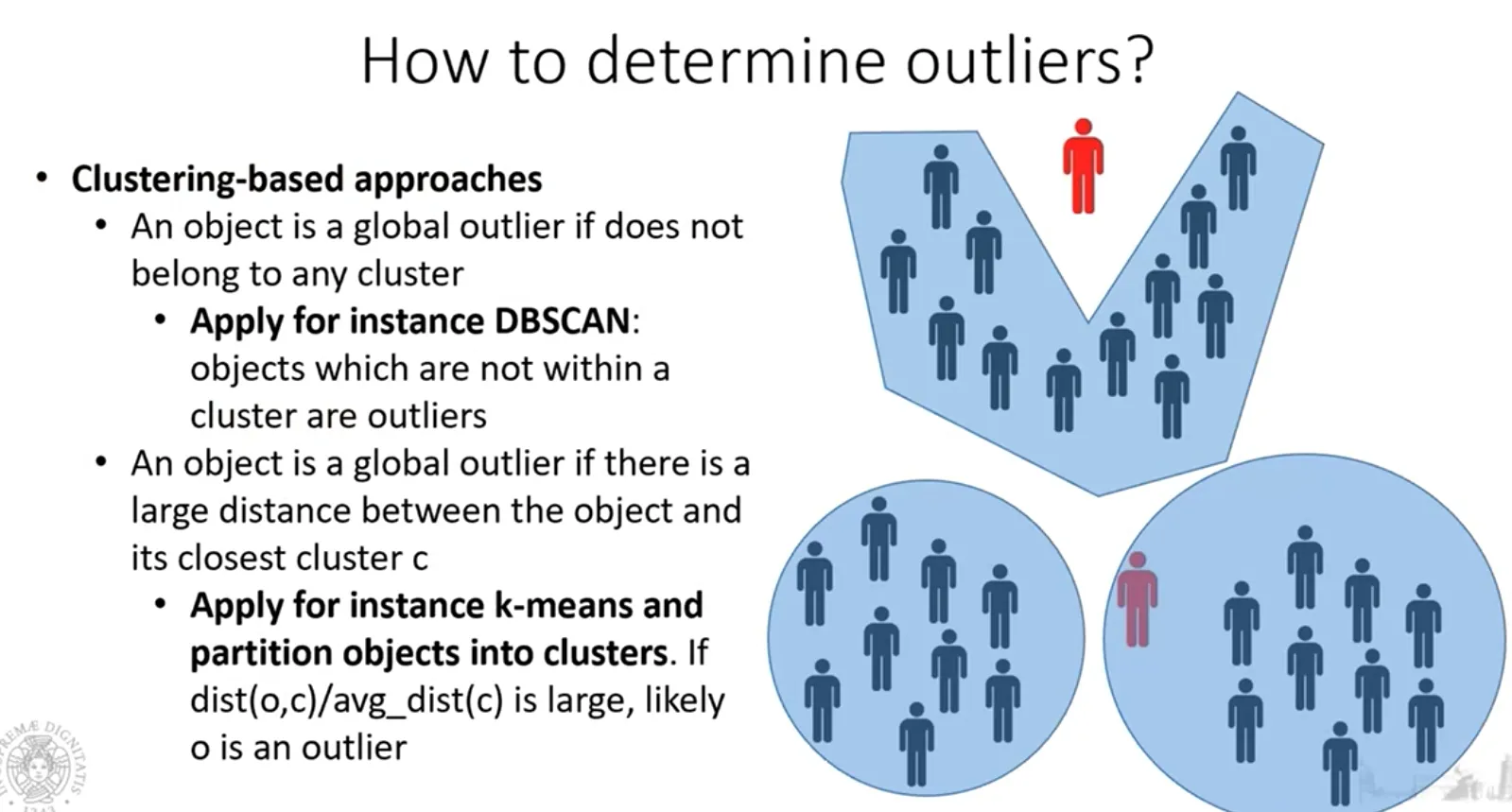
- DBSCAN can find outliers (noise objects), but it was designed to find clusters: finding outliers is a side effect.
- K-means can also be used: run it with a given and, for each point, compare its distance from the centroid with the average distance of the other points of the cluster from the centroid. If this ratio is large, the point is very different from the others and is an outlier.
Both approaches require parameters: Eps and MinPts for DBSCAN; for k-means, besides , a threshold above which the ratio is considered large.
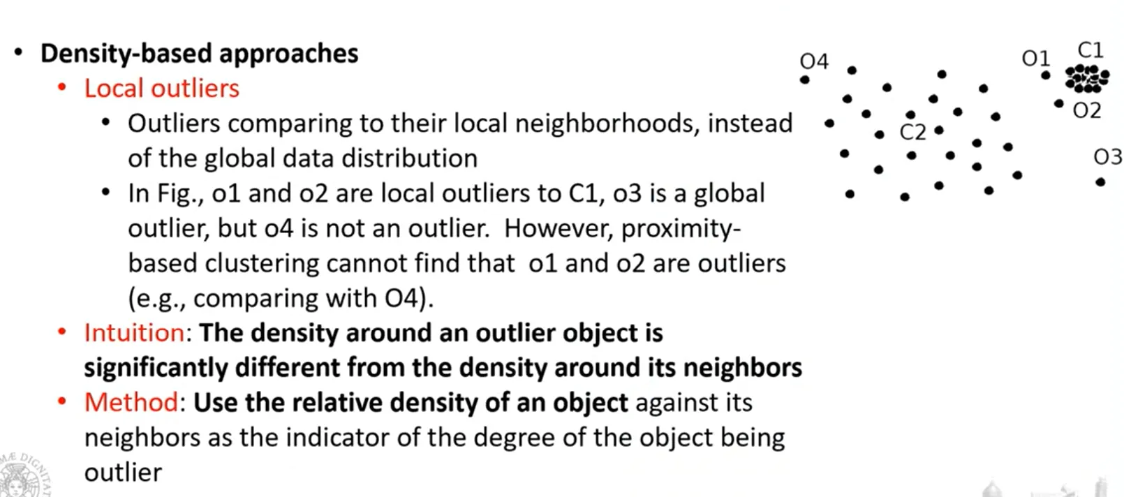
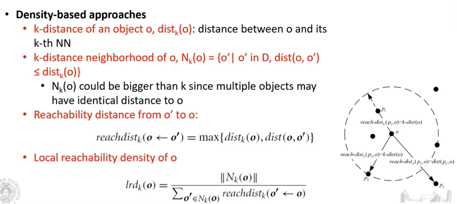
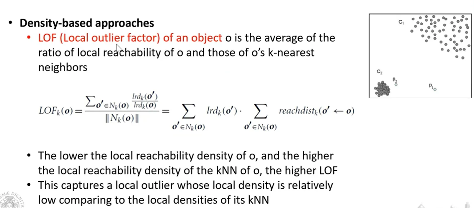
Density-based approach
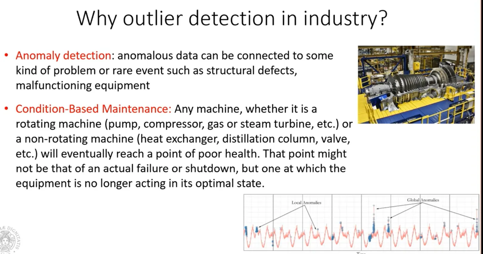
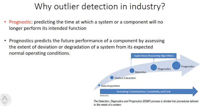
Why outlier detection matters
Frequent Pattern Analysis